Random Fourier Features for Kernel Density Estimation

Home > Estimation > Random Fourier Features for Kernel Density Estimation

Random Fourier Features for Kernel Density Estimation

October 4, 2010 mlstat Leave a comment Go to comments

The NIPS paper Random Fourier Features for Large-scale Kernel Machines, by Rahimi and Recht presents a method for randomized feature mapping where dot products in the transformed feature space approximate (a certain class of) positive definite (p.d.) kernels in the original space.

We know that for any p.d. kernel there exists a deterministic map that has the aforementioned property but it may be infinite dimensional. The paper presents results indicating that with the randomized map we can get away with only a “small” number of features (at least for a classification setting).

Before applying the method to density estimation let us review the relevant section of the paper briefly.

Bochner’s Theorem and Random Fourier Features

Assume that we have data in $R^d$ and a continuous p.d. kernel $K(x,y)$ defined for every pair of points $x,y \in R^d$ . Assume further that the kernel is shift-invariant, i.e., $K(x,y) = K(x-y) \triangleq K(\delta)$ and that the kernel is scaled so that $K(0) = 1$ .

The theorem by Bochner states that under the above conditions $K(\delta)$ must be the Fourier transform of a non-negative measure on $R^d$ . In other words, there exists a probability density function $p(\delta)$ for $\delta \in R^d$ such that $K(\delta) = \mathcal{F}(p(\delta))$ .

where (1) is because $K(.)$ is real. Equation (2) says that if we draw a random vector $w$ according to $p(w)$ and form two vectors $\phi(x) = (cos(w^T x), sin(w^T x))$ and $\phi(y) = (cos(w^T y), sin(w^T y))$ , then the expected value of $<\phi(x),\phi(y)>$ is $K(x-y)$ .

Therefore, for $x \in R^d$ , if we choose the transformation

$\phi(x) = \frac{1}{\sqrt{D}} (cos(w_1^T x), sin(w_1^T x), cos(w_2^T x), sin(w_2^T x), \ldots, cos(w_D^T x), sin(w_D^T x))$

with $w_1,\ldots, w_D$ drawn according to $p(w)$ , linear inner products in this transformed space will approximate $K(.)$ .

Gaussian RBF Kernel

The Gaussian radial basis function kernel satisfies all the above conditions and we know that the Fourier transform of the Gaussian is another Gaussian (with the reciprocal variance). Therefore for “linearizing” the Gaussian r.b.f. kernel, we draw $D$ samples from a Gaussian distribution for the transformation.

Parzen Window Density Estimation

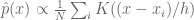
Given a data set $\{x_1, x_2, \ldots, x_N\} \subset R^d$ , the the so-called Parzen window probability density estimator is defined as follows

$\hat{p}(x) \propto \frac{1}{N} \sum_i K((x-x_i)/h)$

where $K(.)$ is often a positive, symmetric, shift-invariant kernel and $h$ is the bandwidth parameter that controls the scale of influence of the data points.

A common kernel that is used for Parzen window density estimation is the Gaussian density. If we make the same choice we can apply our feature transformation to linearize the procedure. We have

where $h$ has been absorbed into the kernel variance.

Therefore all we need to do is take the mean of the transformed data points and estimate the pdf at a new point to be (proportional to) the inner product its transformed feature vector with the mean.

Of course since the kernel value is only approximated by the inner product of the random Fourier features we expect that the estimate pdf will differ from a plain unadorned Parzen window estimate. But different how?

Experiments

Below are some pictures showing how the method performs on some synthetic data. I generated a few dozen points from a mixture of Gaussians and plotted contours of the estimated pdf for the region around the points. I did this for several choices of $D$ and $\gamma$ (the scale parameter for the Gaussian kernel).

First let us check that the method performs as expected for large values of $D$ because the kernel value is well approximated by the inner product of the Fourier features. The first 3 pictures are for $D = 10000$ for various values of $\gamma$ .

D = 10000 and gamma = 2.0

D = 10000 and gamma = 1.0

D = 10000 and gamma = 0.5

—————————————————————————

Now let us see what happens when we decrease $D$ . We expect the error in approximating the kernel would lead to obviously erroneous pdf. This is clearly evident for the case of $D=100$ .

D=1000 and gamma = 1.0

D=100 and gamma = 1.0

—————————————————————————

The following picture for $D = 1000$ and $\gamma = 2.0$ is even stranger.

D = 1000 and gamma = 2.0

—————————————————————————

Discussion

It seems that even for a simple 2D example, we seem to need to compute a very large number of random Fourier features to make the estimated pdf accurate. (For this small example this is very wasteful, since a plain Parzen window estimate would require less memory and computation.)

However, the pictures do indicate that if the approach is to be used for outlier detection (aka novelty detection) from a given data set, we might be able get away with much smaller $D$ . That is, even if the estimated pdf has a big error on the entire space, on the points from the data it seems to be reasonably accurate.

Categories: Estimation Tags: Bochner's theorem, density estimation, Gaussian kernel, novelty detection, outlier detection, Parzen window, Random Fourier Features

Comments (4) Trackbacks (0) Leave a comment Trackback

Manu N

August 1, 2012 at 1:31 pm

Thank you. I was having some trouble understanding this paper
Seungwoo Yoo

September 17, 2013 at 10:41 pm

Thanks a lot it really helps to understand the paper.
Murtaza

November 24, 2015 at 3:27 pm

thanks a lot. IT would have been great if you can share the code.
Murtaza

November 27, 2015 at 12:16 pm

Thanks a lot. It was really easy to understand. Can you please upload your codes too.
Thanks

No trackbacks yet.

The Cult of Universality in Statistical Learning Theory Regularized Minimax on Synthetic Data

Innuo